Basin stability

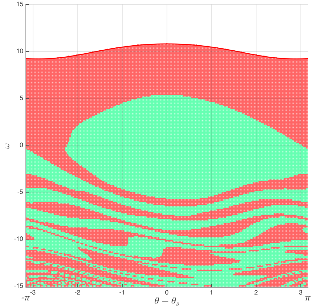
What do you see in the picture? Actually, as it usually happens in science, you see nature. In this case – the basin stability of a one-node power system, where green nodes stand for the regimes that fall into the attractor of the synchronous state.

As part of the Numerical Methods course led by prof. Aslan Kasimov, I studied the synchronization models of power systems and implemented the basin stability, a prominent concept introduced by Peter Menck et al. Explicit Runge-Kutta methods were used to solve the initial value problem posed by the classical swing equation system. It was found that the accuracy and the time step of the methods may significantly influence the estimation of the system’s stability. Convergence analysis of the errors showed that it is preferable to use higher order Runge-Kutta methods to reach a better balance between accuracy and computational cost. The complete report may be found here:
http://materials.andreychurkin.ru/Churkin%20project%20v2.4%2004.04.2020.pdf

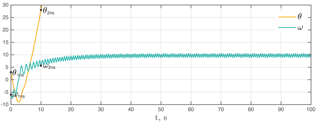
In short, there are two possible outcomes of an electromechanical dynamic process caused by a large perturbation in the system: synchronization (generator’s angular frequency settles to a constant value) or loss of synchrony (generator accelerates until reaching the non-synchronous limit cycle). The following figures show how these outcomes depend on initial conditions.

Synchronization after the initial regime:

Loss of synchronization after the initial regime:

There is a systematic way of analyzing system stability: running numerous simulations with different initial conditions and calculating the basin stability – the ratio of the regimes that lead to the synchronous state to all possible initial conditions in the considered range. So, what you see in the figure below is the result of 40 401 simulations, where the green points depict synchronous states, and red points – loss of synchronization. The stability index, in this case, reaches 38%.

The solutions from the previous simulations can also be represented as trajectories in the stability basin. For example, the regime “1s” leads to a synchronous state where the solution reaches the major green region and starts swinging towards its center. The “1ns” initial values make the generator accelerating up to point “2ns” and further up to the non-synchronous limit cycle.

What else can we see using the basin stability concept? Well, we can play with the model and double the transmission capacity. In this case, the basin will significantly increase, and the stability index would reach 54%:

To further analyze the convergence of the explicit multistage methods for the dynamic power grid model, we estimated the initial stability basin but using an algorithm with a coarse time step. The modified basin got significantly deformed, especially at the bottom of the figure:

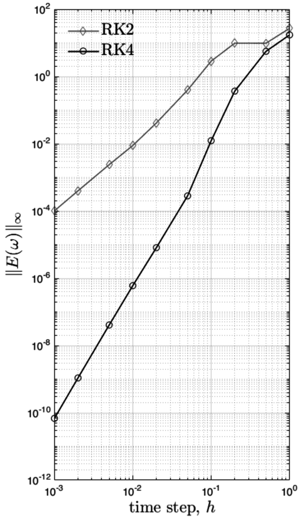
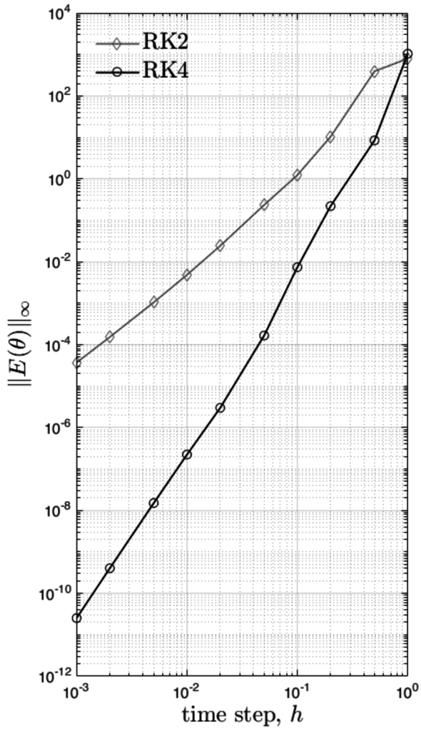
The modified stability index changed to 41%. So, the method with a coarse time step underestimated some oscillations and mistakenly enlarged the stability region. In the report, we performed a complete convergence analysis of the Runge-Kutta methods and concluded that higher order methods are superior in terms of accuracy/cost balance.

Error estimation of the methods:

• 

• 

I am grateful to prof. Aslan Kasimov, who recommended me investigating the oscillator networks and shared the paper by P. Menck on basin stability. This was a hard but entertaining journey.

Andrey Churkin (Андрей Чуркин) 2020